Manual: Concepts
Contents |
Background
Here is where I will write some background information about rigid body dynamics and simulation. But in the meantime, please refer to Baraff's excellent SIGGRAPH tutorial.
Rigid bodies
A rigid body has various properties from the point of view of the simulation. Some properties change over time:
- Position vector (x,y,z) of the body's point of reference. Currently the point of reference must correspond to the body's center of mass.
- Linear velocity of the point of reference, a vector (vx,vy,vz).
- Orientation of a body, represented by a quaternion (qs,qx,qy,qz) or a 3x3 rotation matrix.
- Angular velocity vector (wx,wy,wz) which describes how the orientation changes over time.
Other body properties are usually constant over time:
- Mass of the body.
- Position of the center of mass with respect to the point of reference. In the current implementation the center of mass and the point of reference must coincide.
- Inertia matrix. This is a 3x3 matrix that describes how the body's mass is distributed around the center of mass. Conceptually each body has an x-y-z coordinate frame embedded in it, that moves and rotates with the body, as shown in figure 1.
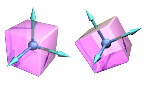
Figure 1: The body coordinate frame.
The origin of this coordinate frame is the body's point of reference. Some values in ODE (vectors, matrices etc) are relative to the body coordinate frame, and others are relative to the global coordinate frame.
Note that the shape of a rigid body is not a dynamical property (except insofar as it influences the various mass properties). It is only collision detection that cares about the detailed shape of the body.
Islands and Disabled Bodies
Bodies are connected to each other with joints. An "island" of bodies is a group that can not be pulled apart - in other words each body is connected somehow to every other body in the island.
Each island in the world is treated separately when the simulation step is taken. This is useful to know: if there are N similar islands in the simulation then the step computation time will be O(N).
Each body can be enabled or disabled. Disabled bodies are effectively "turned off" and are not updated during a simulation step. Disabling bodies is an effective way to save computation time when it is known that the bodies are motionless or otherwise irrelevant to the simulation.
If there are any enabled bodies in an island then every body in the island will be enabled at the next simulation step. Thus to effectively disable an island of bodies, every body in the island must be disabled. If a disabled island is touched by another enabled body then the entire island will be enabled, as a contact joint will join the enabled body to the island.
Integration
The process of simulating the rigid body system through time is called integration. Each integration step advances the current time by a given step size, adjusting the state of all the rigid bodies for the new time value. There are two main issues to consider when working with any integrator:
- How accurate is it? That is, how closely does the behavior of the simulated system match what would happen in real life?
- How stable is it? That is, will calculation errors ever cause completely non-physical behavior of the simulated system? (e.g. causing the system to "explode" for no reason).
ODE's current integrator is very stable, but not particularly accurate unless the step size is small. For most uses of ODE this is not a problem -- ODE's behavior still looks perfectly physical in almost all cases. However ODE should not be used for quantitative engineering until this accuracy issue has been addressed in a future release.
Force accumulators
Between each integrator step the user can call functions to apply forces to the rigid body. These forces are added to "force accumulators" in the rigid body object. When the next integrator step happens, the sum of all the applied forces will be used to push the body around. The forces accumulators are set to zero after each integrator step.
Joints and constraints
In real life a joint is something like a hinge, that is used to connect two objects. In ODE a joint is very similar: It is a relationship that is enforced between two bodies so that they can only have certain positions and orientations relative to each other. This relationship is called a constraint -- the words joint and constraint are often used interchangeably. Figure 2 shows three different constraint types.

Figure 2: Three different constraint types.
The first is a ball and socket joint that constraints the ``ball of one body to be in the same location as the "socket" of another body. The second is a hinge joint that constraints the two parts of the hinge to be in the same location and to line up along the hinge axle. The third is a slider joint that constraints the "piston" and "socket" to line up, and additionally constraints the two bodies to have the same orientation.
Each time the integrator takes a step all the joints are allowed to apply constraint forces to the bodies they affect. These forces are calculated such that the bodies move in such a way to preserve all the joint relationships.
Each joint has a number of parameters controlling its geometry. An example is the position of the ball-and-socket point for a ball-and-socket joint. The functions to set joint parameters all take global coordinates, not body-relative coordinates. A consequence of this is that the rigid bodies that a joint connects must be positioned correctly before the joint is attached.
Joint groups
A joint group is a special container that holds joints in a world. Joints can be added to a group, and then when those joints are no longer needed the entire group of joints can be very quickly destroyed with one function call. However, individual joints in a group can not be destroyed before the entire group is emptied.
This is most useful with contact joints, which are added and remove from the world in groups every time step.
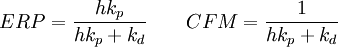
Joint error and the Error Reduction Parameter (ERP)
When a joint attaches two bodies, those bodies are required to have certain positions and orientations relative to each other. However, it is possible for the bodies to be in positions where the joint constraints are not met. This "joint error" can happen in two ways:
- If the user sets the position/orientation of one body without correctly setting the position/orientation of the other body.
- During the simulation, errors can creep in that result in the bodies drifting away from their required positions.
Figure 3 shows an example of error in a ball and socket joint (where the ball and socket do not line up).
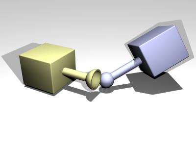
Figure 3: An example of error in a ball and socket joint.
There is a mechanism to reduce joint error: during each simulation step each joint applies a special force to bring its bodies back into correct alignment. This force is controlled by the error reduction parameter (ERP), which has a value between 0 and 1.
The ERP specifies what proportion of the joint error will be fixed during the next simulation step. If ERP=0 then no correcting force is applied and the bodies will eventually drift apart as the simulation proceeds. If ERP=1 then the simulation will attempt to fix all joint error during the next time step. However, setting ERP=1 is not recommended, as the joint error will not be completely fixed due to various internal approximations. A value of ERP=0.1 to 0.8 is recommended (0.2 is the default).
A global ERP value can be set that affects most joints in the simulation. However some joints have local ERP values that control various aspects of the joint.
Soft constraint and Constraint Force Mixing (CFM)
Most constraints are by nature "hard". This means that the constraints represent conditions that are never violated. For example, the ball must always be in the socket, and the two parts of the hinge must always be lined up. In practice constraints can be violated by unintentional introduction of errors into the system, but the error reduction parameter can be set to correct these errors.
Not all constraints are hard. Some "soft" constraints are designed to be violated. For example, the contact constraint that prevents colliding objects from penetrating is hard by default, so it acts as though the colliding surfaces are made of steel. But it can be made into a soft constraint to simulate softer materials, thereby allowing some natural penetration of the two objects when they are forced together.
There are two parameters that control the distinction between hard and soft constraints. The first is the error reduction parameter (ERP) that has already been introduced. The second is the constraint force mixing (CFM) value, that is described below.
Constraint Force Mixing (CFM)
What follows is a somewhat technical description of the meaning of CFM. If you just want to know how it is used in practice then skip to the next section.
Traditionally the constraint equation for every joint has the form

where  is a velocity vector for the bodies involved,
  is a "Jacobian" matrix with one row for every degree of freedom the joint removes from the system, and
  is a right hand side vector. At the next time step, a vector
  is calculated (of the same size as ) such that the forces applied to the bodies to preserve the joint constraint are:

ODE adds a new twist. ODE's constraint equation has the form
where CFM is a square diagonal matrix. CFM mixes the resulting constraint force in with the constraint that produces it. A nonzero (positive) value of CFM allows the original constraint equation to be violated by an amount proportional to CFM times the restoring force that is needed to enforce the constraint. Solving for gives
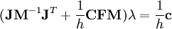
Thus CFM simply adds to the diagonal of the original system matrix. Using a positive value of CFM has the additional benefit of taking the system away from any singularity and thus improving the factorizer accuracy.
How To Use ERP and CFM
ERP and CFM can be independently set in many joints. They can be set in contact joints, in joint limits and various other places, to control the spongyness and springyness of the joint (or joint limit).
If CFM is set to zero, the constraint will be hard. If CFM is set to a positive value, it will be possible to violate the constraint by "pushing on it" (for example, for contact constraints by forcing the two contacting objects together). In other words the constraint will be soft, and the softness will increase as CFM increases. What is actually happening here is that the constraint is allowed to be violated by an amount proportional to CFM times the restoring force that is needed to enforce the constraint. Note that setting CFM to a negative value can have undesirable bad effects, such as instability. Don't do it.
By adjusting the values of ERP and CFM, you can achieve various effects. For example you can simulate springy constraints, where the two bodies oscillate as though connected by springs. Or you can simulate more spongy constraints, without the oscillation. In fact, ERP and CFM can be selected to have the same effect as any desired spring and damper constants. If you have a spring constant  and damping constant
  , then the corresponding ODE constants are:
where  is the step size. These values will give the same effect as a spring-and-damper system simulated with implicit first order integration.
Increasing CFM, especially the global CFM, can reduce the numerical errors in the simulation. If the system is near-singular, then this can markedly increase stability. In fact, if the system is mis-behaving, one of the first things to try is to increase the global CFM.
Collision handling
There is a lot that needs to be written about collision handling.
Collisions between bodies or between bodies and the static environment are handled as follows:
- Before each simulation step, the user calls collision detection functions to determine what is touching what. These functions return a list of contact points. Each contact point specifies a position in space, a surface normal vector, and a penetration depth.
- A special contact joint is created for each contact point. The contact joint is given extra information about the contact, for example the friction present at the contact surface, how bouncy or soft it is, and various other properties.
- The contact joints are put in a joint "group", which allows them to be added to and removed from the system very quickly. The simulation speed goes down as the number of contacts goes up, so various strategies can be used to limit the number of contact points.
- A simulation step is taken.
- All contact joints are removed from the system.
Note that the built-in collision functions do not have to be used - other collision detection libraries can be used as long as they provide the right kinds of contact point information.
Typical simulation code
A typical simulation will proceed like this:
- Create a dynamics world.
- Create bodies in the dynamics world.
- Set the state (position etc) of all bodies.
- Create joints in the dynamics world.
- Attach the joints to the bodies.
- Set the parameters of all joints.
- Create a collision world and collision geometry objects, as necessary.
- Create a joint group to hold the contact joints.
- Loop:
- Apply forces to the bodies as necessary.
- Adjust the joint parameters as necessary.
- Call collision detection.
- Create a contact joint for every collision point, and put it in the contact joint group.
- Take a simulation step.
- Remove all joints in the contact joint group.
- Destroy the dynamics and collision worlds.
Physics model
The various methods and approximations that are used in ODE are discussed here.
Friction Approximation
We really need more pictures here.
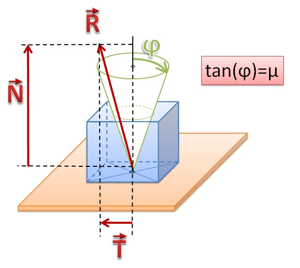
Figure: Angle of friction.
The Coulomb friction model is a simple, but effective way to model friction at contact points. It is a simple relationship between the normal and tangential forces present at a contact point (see the contact joint section for a description of these forces). The rule is:
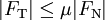
where  and
and  are the normal and tangential force vectors respectively, and
  is the friction coefficient (typically a number around 1.0). This equation defines a "friction cone" - imagine a cone with
  as the axis and the contact point as the vertex. If the total friction force vector is within the cone then the contact is in "sticking mode", and the friction force is enough to prevent the contacting surfaces from moving with respect to each other. If the force vector is on the surface of the cone then the contact is in "sliding mode", and the friction force is typically not large enough to prevent the contacting surfaces from sliding. The parameter thus specifies the maximum ratio of tangential to normal force.
ODE's friction models are approximations to the friction cone, for reasons of efficiency. There are currently two approximations to chose from:
- The meaning of is changed so that it specifies the maximum friction (tangential) force that can be present at a contact, in either of the tangential friction directions. This is rather non physical because it is independent of the normal force, but it can be useful and it is the computationally cheapest option. Note that in this case is a force limit an must be chosen appropriate to the simulation.
- The friction cone is approximated by a friction pyramid aligned with the first and second friction directions (I really need a picture here). A further approximation is made: first ODE computes the normal forces assuming that all the contacts are frictionless. Then it computes the maximum limits
 for the friction (tangential) forces from

and then proceeds to solve for the entire system with these fixed limits (in a manner similar to approximation 1 above). This differs from a true friction pyramid in that the "effective" mu is not quite fixed. This approximation is easier to use as is a unit-less ratio the same as the normal Coloumb friction coefficient, and thus can be set to a constant value around 1.0 without regard for the specific simulation.