The Open Dynamics Engine (ODE) is a free, industrial quality library for simulating articulated rigid body dynamics. For example, it is good for simulating ground vehicles, legged creatures, and moving objects in VR environments. It is fast, flexible and robust, and it has built-in collision detection. ODE is being developed by Russell Smith with help from several contributors.
If ``rigid body simulation'' does not make much sense to you, check out What is a Physics SDK?.
This is the user guide for ODE version 0.039. Despite the low version number, ODE is reasonably mature and stable.
ODE is best for simulating articulated rigid body structures. An articulated structure is created when rigid bodies of various shapes are connected together with joints of various kinds. Examples are ground vehicles (where the wheels are connected to the chassis), legged creatures (where the legs are connected to the body), or stacks of objects.
ODE is designed to be used in interactive or real-time simulation. It is particularly good for simulating moving objects in changeable virtual reality environments. This is because it is fast, robust and stable, and the user has complete freedom to change the structure of the system even while the simulation is running.
ODE uses a highly stable integrator, so that the simulation errors should not grow out of control. The physical meaning of this is that the simulated system should not "explode" for no reason (believe me, this happens a lot with other simulators if you are not careful). ODE emphasizes speed and stability over physical accuracy.
ODE has hard contacts. This means that a special non-penetration constraint is used whenever two bodies collide. The alternative, used in many other simulators, is to use virtual springs to represent contacts. This is difficult to do right and extremely error-prone.
ODE has a built-in collision detection system. However you can ignore it and do your own collision detection if you want to. The current collision primitives are sphere, box, capped cylinder, plane, ray, and triangular mesh - more collision objects will come later. ODE's collision system provides fast identification of potentially intersecting objects, through the concept of ``spaces''.
Here are the features:
ODE is Copyright © 2001-2003 Russell L. Smith. All rights reserved.
This library is free software; you can redistribute it and/or modify it under the terms of EITHER:
Do you have questions or comments about ODE? Think you can help? Please write to the ODE mailing list.
Step 1: Unpack the ODE archive.
Step 2: Get the GNU make tool. Many Unix platforms come with this, although sometimes it is called gmake. I have provided a version of GNU make for windows here.
Step 3: Edit the settings in the file config/user-settings. The list of supported platforms is given in that file.
Step 4: Run make to configure and build ODE and the graphical test programs. Be sure you are using the correct version of GNU make. The make targets for building the parts of ODE are:
Step 5: To install the ODE library onto your system you should copy the lib/ and include/ directories to a suitable place, e.g. on Unix:
There is currently no built-in support to build Windows DLLs or Unix shared libraries --- although it is not hard to add this yourself.
ODE has been verified to build on at least the following platforms:
ODE uses XWindows and OpenGL to render the scene being simulated. In order to build the example you will need to install Apple X11 server and the X11SDK (as well as the normal developer tools).
These are available from Apple. As of writing this can be found at: http://www.apple.com/macosx/x11. NOTE: there is a tiny link at the bottom right of the page for the SDK
Once the software is installed follow the normal build instructions.
Since ODE uses X11 you need to run the X11 server (which you should have installed, it's in the Applications Folder).
If you run the test app in the XTerm that the X11 server opens by default then they should run fine. If however you run them from a MacOS X Terminal then you need to define the enviroment variable DISPLAY. If DISPLAY is not defined then you will get a message saying: "cannot open X11 display".
For example to run the boxstack test you would type
    cd ode/test
    DISPLAY=:0.0 ./test_boxstack.exe
|
The best way to understand how to use ODE is to look at the test/example programs that come with it. Note the following things:
#include <ode/ode.h> |
gcc -c -I /home/username/ode/include myprogram.cpp |
[Here is where I will write some background information about rigid body dynamics and simulation. But in the meantime, please refer to Baraff's excellent SIGGRAPH tutorial].
A rigid body has various properties from the point of view of the simulation. Some properties change over time:
The origin of this coordinate frame is the body's point of reference. Some values in ODE (vectors, matrices etc) are relative to the body coordinate frame, and others are relative to the global coordinate frame.
Note that the shape of a rigid body is not a dynamical property (except insofar as it influences the various mass properties). It is only collision detection that cares about the detailed shape of the body.
Bodies are connected to each other with joints. An ``island'' of bodies is a group that can not be pulled apart - in other words each body is connected somehow to every other body in the island.
Each island in the world is treated separately when the simulation step is taken. This is useful to know: if there are N similar islands in the simulation then the step computation time will be O(N).
Each body can be enabled or disabled. Disabled bodies are effectively ``turned off'' and are not updated during a simulation step. Disabling bodies is an effective way to save computation time when it is known that the bodies are motionless or otherwise irrelevent to the simulation.
If there are any enabled bodies in an island then every body in the island will be enabled at the next simulation step. Thus to effectively disable an island of bodies, every body in the island must be disabled. If a disabled island is touched by another enabled body then the entire island will be enabled, as a contact joint will join the enabled body to the island.
The process of simulating the rigid body system through time is called integration. Each integration step advances the current time by a given step size, adjusting the state of all the rigid bodies for the new time value. There are two main issues to consider when working with any integrator:
Between each integrator step the user can call functions to apply forces to the rigid body. These forces are added to "force accumulators" in the rigid body object. When the next integrator step happens, the sum of all the applied forces will be used to push the body around. The forces accumulators are set to zero after each integrator step.
In real life a joint is something like a hinge, that is used to connect two objects. In ODE a joint is very similar: It is a relationship that is enforced between two bodies so that they can only have certain positions and orientations relative to each other. This relationship is called a constraint -- the words joint and constraint are often used interchangeably. The following picture shows three different constraint types:

The first is a ball and socket joint that constraints the ``ball'' of one body to be in the same location as the ``socket'' of another body. The second is a hinge joint that constraints the two parts of the hinge to be in the same location and to line up along the hinge axle. The third is a slider joint that constraints the ``piston'' and ``socket'' to line up, and additionally constraints the two bodies to have the same orientation.
Each time the integrator takes a step all the joints are allowed to apply constraint forces to the bodies they affect. These forces are calculated such that the bodies move in such a way to preserve all the joint relationships.
Each joint has a number of parameters controlling its geometry. An example is the position of the ball-and-socket point for a ball-and-socket joint. The functions to set joint parameters all take global coordinates, not body-relative coordinates. A consequence of this is that the rigid bodies that a joint connects must be positioned correctly before the joint is attached.
A joint group is a special container that holds joints in a world. Joints can be added to a group, and then when those joints are no longer needed the entire group of joints can be very quickly destroyed with one function call. However, individual joints in a group can not be destroyed before the entire group is emptied.
This is most useful with contact joints, which are added and remove from the world in groups every time step.
When a joint attaches two bodies, those bodies are required to have certain positions and orientations relative to each other. However, it is possible for the bodies to be in positions where the joint constraints are not met. This ``joint error'' can happen in two ways:
There is a mechanism to reduce joint error: during each simulation step each joint applies a special force to bring its bodies back into correct alignment. This force is controlled by the error reduction parameter (ERP), which has a value between 0 and 1.
The ERP specifies what proportion of the joint error will be fixed during the next simulation step. If ERP=0 then no correcting force is applied and the bodies will eventually drift apart as the simulation proceeds. If ERP=1 then the simulation will attempt to fix all joint error during the next time step. However, setting ERP=1 is not recommended, as the joint error will not be completely fixed due to various internal approximations. A value of ERP=0.1 to 0.8 is recommended (0.2 is the default).
A global ERP value can be set that affects most joints in the simulation. However some joints have local ERP values that control various aspects of the joint.
Most constraints are by nature ``hard''. This means that the constraints represent conditions that are never violated. For example, the ball must always be in the socket, and the two parts of the hinge must always be lined up. In practice constraints can be voilated by unintentional introduction of errors into the system, but the error reduction parameter can be set to correct these errors.
Not all constraints are hard. Some ``soft'' constraints are designed to be violated. For example, the contact constraint that prevents colliding objects from penetrating is hard by default, so it acts as though the colliding surfaces are made of steel. But it can be made into a soft constraint to simulate softer materials, thereby allowing some natural penetration of the two objects when they are forced together.
There are two parameters that control the distinction between hard and soft constraints. The first is the error reduction parameter (ERP) that has already been introduced. The second is the constraint force mixing (CFM) value, that is described below.
What follows is a somewhat technical description of the meaning of CFM. If you just want to know how it is used in practice then skip to the next section.
Traditionally the constraint equation for every joint has the form
where v is a velocity vector for the bodies involved, J is a ``Jacobian'' matrix with one row for every degree of freedom the joint removes from the system, and c is a right hand side vector. At the next time step, a vector lambda is calculated (of the same size as c) such that the forces applied to the bodies to preserve the joint constraint are
ODE adds a new twist. ODE's constraint equation has the form
where CFM is a square diagonal matrix. CFM mixes the resulting constraint force in with the constraint that produces it. A nonzero (positive) value of CFM allows the original constraint equation to be violated by an amount proportional to CFM times the restoring force lamda that is needed to enforce the constraint. Solving for lambda gives
Thus CFM simply adds to the diagonal of the original system matrix. Using a positive value of CFM has the additional benefit of taking the system away from any singularity and thus improving the factorizer accuracy.
ERP and CFM can be independently set in many joints. They can be set in contact joints, in joint limits and various other places, to control the spongyness and springyness of the joint (or joint limit).
If CFM is set to zero, the constraint will be hard. If CFM is set to a positive value, it will be possible to violate the constraint by ``pushing on it'' (for example, for contact constraints by forcing the two contacting objects together). In other words the constraint will be soft, and the softness will increase as CFM increases. What is actually happeneng here is that the constraint is allowed to be violated by an amount proportional to CFM times the restoring force that is needed to enforce the constraint. Note that setting CFM to a negative value can have undesirable bad effects, such as instability. Don't do it.
By adjusting the values of ERP and CFM, you can achieve various effects. For example you can simulate springy constraints, where the two bodies oscillate as though connected by springs. Or you can simulate more spongy constraints, without the oscillation. In fact, ERP and CFM can be selected to have the same effect as any desired spring and damper constants. If you have a spring constant kp and damping constant kd, then the corresponding ODE constants are:
where h is the stepsize. These values will give the same effect as a spring-and-damper system simulated with implicit first order integration.
Increasing CFM, especially the global CFM, can reduce the numerical errors in the simulation. If the system is near-singular, then this can markedly increase stability. In fact, if the system is mis-behaving, one of the first things to try is to increase the global CFM.
[There is a lot that needs to be written about collision handling.]
Collisions between bodies or between bodies and the static environment are handled as follows:
A typical simulation will proceed like this:
The various methods and approximations that are used in ODE are discussed here.
[We really need more pictures here.]
The Coulomb friction model is a simple, but effective way to model friction at contact points. It is a simple relationship between the normal and tangential forces present at a contact point (see the contact joint section for a description of these forces). The rule is:
where fN and fT are the normal and tangential force vectors respectively, and mu is the friction coefficient (typically a number around 1.0). This equation defines a "friction cone" - imagine a cone with fN as the axis and the contact point as the vertex. If the total friction force vector is within the cone then the contact is in "sticking mode", and the friction force is enough to prevent the contacting surfaces from moving with respect to each other. If the force vector is on the surface of the cone then the contact is in "sliding mode", and the friction force is typically not large enough to prevent the contacting surfaces from sliding. The parameter mu thus specifies the maximum ratio of tangential to normal force.
ODE's friction models are approximations to the friction cone, for reasons of efficiency. There are currently two approximations to chose from:
and then proceeds to solve for the entire system with these fixed limits (in a manner similar to approximation 1 above). This differs from a true friction pyramid in that the "effective" mu is not quite fixed. This approximation is easier to use as mu is a unitless ratio the same as the normal Coloumb friction coefficient, and thus can be set to a constant value around 1.0 without regard for the specific simulation.
The ODE library can be built to use either single or double precision floating point numbers. Single precision is faster and uses less memory, but the simulation will have more numerical error that can result in visible problems. You will get less accuracy and stability with single precision.
[must describe what factors influence accuracy and stability].
The floating point data type is dReal. Other commonly used types are dVector3, dVector4, dMatrix3, dMatrix4, dQuaternion.
There are various kinds of object that can be created:
All 3-vectors (x,y,z) supplied to ``set'' functions are given as individual x,y,z arguments.
All 3-vector result arguments to get() function are pointers to arrays of dReal.
Larger vectors are always supplied and returned as pointers to arrays of dReal.
All coordinates are in the global frame except where otherwise specified.
The ODE library is written in C++, but its public interface is made of simple C functions, not classes. Why is this?
The ODE library can be compiled in "debugging" or "release" mode. Debugging mode is slower, but function arguments are checked and many run-time tests are done to ensure internal consistency. Release mode is faster, but no checking is done.
The world object is a container for rigid bodies and joints. Objects in different worlds can not interact, for example rigid bodies from two different worlds can not collide.
All the objects in a world exist at the same point in time, thus one reason to use separate worlds is to simulate systems at different rates.
Most applications will only need one world.
dWorldID dWorldCreate();
Create a new, empty world and return its ID number.
void dWorldDestroy (dWorldID);
Destroy a world and everything in it. This includes all bodies, and all
joints that are not part of a joint group.
Joints that are part of a joint group will be deactivated, and can be
destroyed by calling, for example, dJointGroupEmpty().
void dWorldSetGravity (dWorldID, dReal x, dReal y, dReal z);
void dWorldGetGravity (dWorldID, dVector3 gravity);
Set and get the world's global gravity vector. The units are m/s/s, so Earth's
gravity vector would be (0,0,-9.81), assuming that +z is up.
The default is no gravity, i.e. (0,0,0).
void dWorldSetERP (dWorldID, dReal erp);
dReal dWorldGetERP (dWorldID);
Set and get the global ERP value, that controls how much error correction is
performed in each time step.
Typical values are in the range 0.1--0.8.
The default is 0.2.
void dWorldSetCFM (dWorldID, dReal cfm);
dReal dWorldGetCFM (dWorldID);
Set and get the global CFM (constraint force mixing) value.
Typical values are in the range 1e-9 -- 1.
The default is 1e-5 if single precision is being used, or 1e-10 if double
precision is being used.
void dWorldStep (dWorldID, dReal stepsize);
Step the world.
This function is given the desired impulse as (ix,iy,iz) and puts the force vector in force. The current algorithm simply scales the impulse by 1/stepsize, where stepsize is the step size for the next step that will be taken.
This function is given a dWorldID because, in the future, the force computation may depend on integrator parameters that are set as properties of the world.
void dCloseODE();
This deallocates some extra memory used by ODE that can not be deallocated
using the normal destroy functions, e.g. dWorldDestroy().
You can use this function at the end of your application to prevent
memory leak checkers from complaining about ODE.
void dBodySetPosition   (dBodyID, dReal x, dReal y, dReal z);
void dBodySetRotation   (dBodyID, const dMatrix3 R);
void dBodySetQuaternion (dBodyID, const dQuaternion q);
void dBodySetLinearVel  (dBodyID, dReal x, dReal y, dReal z);
void dBodySetAngularVel (dBodyID, dReal x, dReal y, dReal z);
const dReal * dBodyGetPosition   (dBodyID);
const dReal * dBodyGetRotation   (dBodyID);
const dReal * dBodyGetQuaternion (dBodyID);
const dReal * dBodyGetLinearVel  (dBodyID);
const dReal * dBodyGetAngularVel (dBodyID);
These functions set and get the position, rotation, linear and angular
velocity of the body.
After setting a group of bodies, the outcome of the simulation is undefined
if the new configuration is inconsistent with the joints/constraints that are
present.
When getting, the returned values are pointers to internal data structures,
so the vectors are valid until any changes are made to the rigid body system
structure.
Hmmm. dBodyGetRotation returns a 4x3 rotation matrix.
void dBodySetMass (dBodyID, const dMass *mass);
void dBodyGetMass (dBodyID, dMass *mass);
Set/get the mass of the body (see the mass functions).
void dBodyAddForce            (dBodyID, dReal fx, dReal fy, dReal fz);
void dBodyAddTorque           (dBodyID, dReal fx, dReal fy, dReal fz);
void dBodyAddRelForce         (dBodyID, dReal fx, dReal fy, dReal fz);
void dBodyAddRelTorque        (dBodyID, dReal fx, dReal fy, dReal fz);
void dBodyAddForceAtPos       (dBodyID, dReal fx, dReal fy, dReal fz,
                                        dReal px, dReal py, dReal pz);
void dBodyAddForceAtRelPos    (dBodyID, dReal fx, dReal fy, dReal fz,
                                        dReal px, dReal py, dReal pz);
void dBodyAddRelForceAtPos    (dBodyID, dReal fx, dReal fy, dReal fz,
                                        dReal px, dReal py, dReal pz);
void dBodyAddRelForceAtRelPos (dBodyID, dReal fx, dReal fy, dReal fz,
                                        dReal px, dReal py, dReal pz);
Add forces to bodies (absolute or relative coordinates).
The forces are accumulated on to each body, and the accumulators are zeroed
after each time step.
The ...RelForce and ...RelTorque functions take force vectors that are relative to the body's own frame of reference.
The ...ForceAtPos and ...ForceAtRelPos functions take an extra position vector (in global or body-relative coordinates respectively) that specifies the point at which the force is applied. All other functions apply the force at the center of mass.
const dReal * dBodyGetForce  (dBodyID);
const dReal * dBodyGetTorque (dBodyID);
Return the current accumulated force and torque vector.
The returned pointers point to an array of 3 dReals.
The returned values are pointers to internal data structures, so the vectors
are only valid until any changes are made to the rigid body system.
void dBodySetForce  (dBodyID b, dReal x, dReal y, dReal z);
void dBodySetTorque (dBodyID b, dReal x, dReal y, dReal z);
Set the body force and torque accumulation vectors.
This is mostly useful to zero the force and torque for deactivated bodies
before they are reactivated, in the case where the force-adding functions
were called on them while they were deactivated.
void dBodyGetRelPointPos (dBodyID, dReal px, dReal py, dReal pz,
                          dVector3 result);
void dBodyGetRelPointVel (dBodyID, dReal px, dReal py, dReal pz,
                          dVector3 result);
void dBodyGetPointVel    (dBodyID, dReal px, dReal py, dReal pz,
                          dVector3 result);
Utility functions that take a point on a body (px,py,pz) and
return that point's position or velocity in global coordinates
(in result).
The dBodyGetRelPointXXX functions are given the point in body
relative coordinates, and the dBodyGetPointVel function is given
the point in global coordinates.
void dBodyGetPosRelPoint (dBodyID, dReal px, dReal py, dReal pz,
                       	  dVector3 result);
This is the inverse of dBodyGetRelPointPos().
It takes a point in global coordinates (x,y,z) and returns
the point's position in body-relative coordinates (result).
void dBodyVectorToWorld   (dBodyID, dReal px, dReal py, dReal pz,
                           dVector3 result);
void dBodyVectorFromWorld (dBodyID, dReal px, dReal py, dReal pz,
                           dVector3 result);
Given a vector expressed in the body (or world) coordinate system
(x,y,z), rotate it to the world (or body) coordinate system
(result).
void  dBodySetData (dBodyID, void *data);
void *dBodyGetData (dBodyID);
Get and set the body's user-data pointer.
void dBodyEnable (dBodyID);
void dBodyDisable (dBodyID);
int dBodyIsEnabled (dBodyID);
Enable and disable a body.
Disabled bodies are effectively ``turned off'' and are not updated during a
simulation step.
However, if a disabled body is connected to an island containing one or more
enabled bodies then it will be re-enabled at the next simulation step.
dBodyIsEnabled() returns 1 if a body is enabled or 0 if it is disabled. New bodies are created in the enabled state.
void dBodySetFiniteRotationAxis (dBodyID, dReal x, dReal y, dReal z);
This sets the finite rotation axis for a body.
This is axis only has meaning when the finite rotation mode is set
(see dBodySetFiniteRotationMode()).
If this axis is zero (0,0,0), full finite rotations are performed on the body.
If this axis is nonzero, the body is rotated by performing a partial finite rotation along the axis direction followed by an infitesimal rotation along an orthogonal direction.
This can be useful to alleviate certain sources of error caused by quickly spinning bodies. For example, if a car wheel is rotating at high speed you can call this function with the wheel's hinge axis as the argument to try and improve its behavior.
int dBodyGetNumJoints (dBodyID b);
Return the number of joints that are attached to this body.
dJointID dBodyGetJoint (dBodyID, int index);
Return a joint attached to this body, given by index.
Valid indexes are 0 to n-1 where n is the value returned by
dBodyGetNumJoints().
void dBodySetGravityMode (dBodyID b, int mode);
int dBodyGetGravityMode (dBodyID b);
Set/get whether the body is influenced by the world's gravity or not.
If mode is nonzero it is, if mode is zero, it isn't.
Newly created bodies are always influenced by the world's gravity.
dJointID dJointCreateBall (dWorldID, dJointGroupID);
dJointID dJointCreateHinge (dWorldID, dJointGroupID);
dJointID dJointCreateSlider (dWorldID, dJointGroupID);
dJointID dJointCreateContact (dWorldID, dJointGroupID,
                              const dContact *);
dJointID dJointCreateUniversal (dWorldID, dJointGroupID);
dJointID dJointCreateHinge2 (dWorldID, dJointGroupID);
dJointID dJointCreateFixed (dWorldID, dJointGroupID);
dJointID dJointCreateAMotor (dWorldID, dJointGroupID);
Create a new joint of a given type.
The joint is initially in "limbo" (i.e. it has no effect on the simulation)
because it does not connect to any bodies.
The joint group ID is 0 to allocate the joint normally.
If it is nonzero the joint is allocated in the given joint group.
The contact joint will be initialized with the given dContact
structure.
Some joints, like hinge-2 need to be attached to two bodies to work.
void dJointSetData (dJointID, void *data);
void *dJointGetData (dJointID);
Get and set the joint's user-data pointer.
int dJointGetType (dJointID);
Get the joint's type. One of the following constants will be returned:
| dJointTypeBall | A ball-and-socket joint. |
| dJointTypeHinge | A hinge joint. |
| dJointTypeSlider | A slider joint. |
| dJointTypeContact | A contact joint. |
| dJointTypeUniversal | A universal joint. |
| dJointTypeHinge2 | A hinge-2 joint. |
| dJointTypeFixed | A fixed joint. |
| dJointTypeAMotor | An angular motor joint. |
void dJointSetFeedback (dJointID, dJointFeedback *);
dJointFeedback *dJointGetFeedback (dJointID);
During the world time step, the forces that are applied by each joint are
computed. These forces are added directly to the joined bodies, and the user
normally has no way of telling which joint contributed how much force.
If this information is desired then the user can allocate a dJointFeedback structure and pass its pointer to the dJointSetFeedback() function. The feedback information structure is defined as follows:
typedef struct dJointFeedback {
  dVector3 f1;       // force that joint applies to body 1
  dVector3 t1;       // torque that joint applies to body 1
  dVector3 f2;       // force that joint applies to body 2
  dVector3 t2;       // torque that joint applies to body 2
} dJointFeedback;
|
During the time step any feedback structures that are attached to joints will be filled in with the joint's force and torque information. The dJointGetFeedback() function returns the current feedback structure pointer, or 0 if none is used (this is the default). dJointSetFeedback() can be passed 0 to disable feedback for that joint.
Now for some API design notes. It might seem strange to require that users perform the allocation of these structures. Why not just store the data statically in each joint? The reason is that not all users will use the feedback information, and even when it is used not all joints will need it. It will waste memory to store it statically, especially as this structure could grow to store a lot of extra information in the future.
Why not have ODE allocate the structure itself, at the user's request? The reason is that contact joints (which are created and destroyed every time step) would require a lot of time to be spent in memory allocation if feedback is required. Letting the user do the allocation means that a better allocation strategy can be provided, e.g simply allocating them out of a fixed array.
The alternative to this API is to have a joint-force callback. This would work of course, but it has a few problems. First, callbacks tend to pollute APIs and sometimes require the user to go through unnatural contortions to get the data to the right place. Second, this would expose ODE to being changed in the middle of a step (which would have bad consequences), and there would have to be some kind of guard against this or a debugging check for it - which would complicate things.
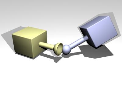
A ball and socket joint looks like this:
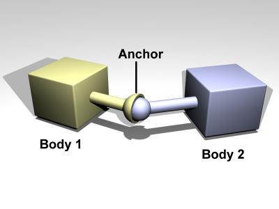
void dJointGetBallAnchor2 (dJointID, dVector3 result);
Get the joint anchor point, in world coordinates. This returns the point on
body 2. You can think of a ball and socket joint as trying to keep the result
of dJointGetBallAnchor() and dJointGetBallAnchor2() the same. If the joint is
perfectly satisfied, this function will return the same value
as dJointGetBallAnchor() to within roundoff errors. dJointGetBallAnchor2()
can be used, along with dJointGetBallAnchor(), to see how far the joint has come apart.
A hinge joint looks like this:
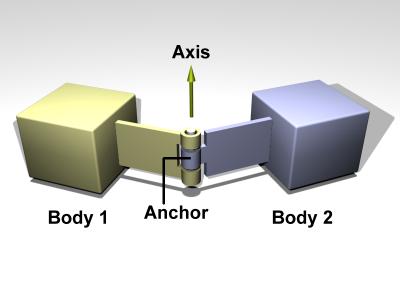
void dJointSetHingeAnchor (dJointID, dReal x, dReal y, dReal z);
void dJointSetHingeAxis (dJointID, dReal x, dReal y, dReal z);
Set hinge anchor and axis parameters.
void dJointGetHingeAnchor2 (dJointID, dVector3 result);
Get the joint anchor point, in world coordinates. This returns the point on
body 2. If the joint is perfectly satisfied, this will return the same value
as dJointGetHingeAnchor(). If not, this value will be slightly different.
This can be used, for example, to see how far the joint has come apart.
void dJointGetHingeAxis (dJointID, dVector3 result);
Get hinge axis parameter.
dReal dJointGetHingeAngle (dJointID);
dReal dJointGetHingeAngleRate (dJointID);
Get the hinge angle and the time derivative of this value.
The angle is measured between the two bodies, or between the body and
the static environment.
The angle will be between -pi..pi.
When the hinge anchor or axis is set, the current position of the attached bodies is examined and that position will be the zero angle.
A slider joint looks like this:
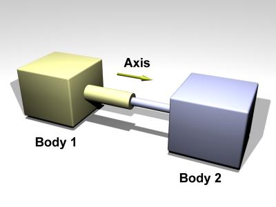
void dJointSetSliderAxis (dJointID, dReal x, dReal y, dReal z);
Set the slider axis parameter.
void dJointGetSliderAxis (dJointID, dVector3 result);
Get the slider axis parameter.
dReal dJointGetSliderPosition (dJointID);
dReal dJointGetSliderPositionRate (dJointID);
Get the slider linear position (i.e. the slider's ``extension'') and the time
derivative of this value.
When the axis is set, the current position of the attached bodies is examined and that position will be the zero position.
A universal joint looks like this:
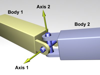
A universal joint is like a ball and socket joint that constrains an extra degree of rotational freedom. Given axis 1 on body 1, and axis 2 on body 2 that is perpendicular to axis 1, it keeps them perpendicular. In other words, rotation of the two bodies about the direction perpendicular to the two axes will be equal.
In the picture, the two bodies are joined together by a cross. Axis 1 is attached to body 1, and axis 2 is attached to body 2. The cross keeps these axes at 90 degrees, so if you grab body 1 and twist it, body 2 will twist as well.
Universal joints show up in cars, where the engine causes a shaft, the drive shaft, to rotate along its own axis. At some point you'd like to change the direction of the shaft. The problem is, if you just bend the shaft, then the part after the bend won't rotate about its own axis. So if you cut it at the bend location and insert a universal joint, you can use the constraint to force the second shaft to rotate about the same angle as the first shaft.
Another use of this joint is to attach the arms of a simple virtual creature to its body. Imagine a person holding their arms straight out. You may want the arm to be able to move up and down, and forward and back, but not to rotate about its own axis.
Here are the universal joint functions:
void dJointSetUniversalAnchor (dJointID, dReal x, dReal y, dReal z);
void dJointSetUniversalAxis1 (dJointID, dReal x, dReal y, dReal z);
void dJointSetUniversalAxis2 (dJointID, dReal x, dReal y, dReal z);
Set universal anchor and axis parameters.
Axis 1 and axis 2 should be perpendicular to each other.
void dJointGetUniversalAnchor2 (dJointID, dVector3 result);
Get the joint anchor point, in world coordinates. This returns the point on
body 2. You can think of the ball and socket part of a universal joint as
trying to keep the result of dJointGetBallAnchor() and dJointGetBallAnchor2()
the same. If the joint is
perfectly satisfied, this function will return the same value
as dJointGetUniversalAnchor() to within roundoff errors. dJointGetUniveralAnchor2()
can be used, along with dJointGetUniversalAnchor(), to see how far the joint has come apart.
void dJointGetUniversalAxis1 (dJointID, dVector3 result);
void dJointGetUniversalAxis2 (dJointID, dVector3 result);
Get univeral axis parameters.
A hinge-2 joint looks like this:
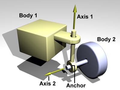
The hinge-2 joint is the same as two hinges connected in series, with different hinge axes. An example, shown in the above picture is the steering wheel of a car, where one axis allows the wheel to be steered and the other axis allows the wheel to rotate.
The hinge-2 joint has an anchor point and two hinge axes. Axis 1 is specified relative to body 1 (this would be the steering axis if body 1 is the chassis). Axis 2 is specified relative to body 2 (this would be the wheel axis if body 2 is the wheel).
Axis 1 can have joint limits and a motor, axis 2 can only have a motor.
Axis 1 can function as a suspension axis, i.e. the constraint can be compressible along that axis.
void dJointSetHinge2Anchor (dJointID, dReal x, dReal y, dReal z);
void dJointSetHinge2Axis1 (dJointID, dReal x, dReal y, dReal z);
void dJointSetHinge2Axis2 (dJointID, dReal x, dReal y, dReal z);
Set hinge-2 anchor and axis parameters.
Axis 1 and axis 2 must not lie along the same line.
void dJointGetHinge2Anchor2 (dJointID, dVector3 result);
Get the joint anchor point, in world coordinates. This returns the point on
body 2. If the joint is perfectly satisfied, this will return the same value
as dJointGetHinge2Anchor(). If not, this value will be slightly different.
This can be used, for example, to see how far the joint has come apart.
void dJointGetHinge2Axis1 (dJointID, dVector3 result);
void dJointGetHinge2Axis2 (dJointID, dVector3 result);
Get hinge-2 axis parameters.
dReal dJointGetHinge2Angle1 (dJointID);
dReal dJointGetHinge2Angle1Rate (dJointID);
dReal dJointGetHinge2Angle2Rate (dJointID);
Get the hinge-2 angles (around axis 1 and axis 2) and the time derivatives
of these values.
When the anchor or axis is set, the current position of the attached bodies is examined and that position will be the zero angle.
The fixed joint maintains a fixed relative position and orientation between two bodies, or between a body and the static environment. Using this joint is almost never a good idea in practice, except when debugging. If you need two bodies to be glued together it is better to represent that as a single body.
Currently the fixed joint does not support a non-identity relative rotation between two bodies, it only supports a relative offset.
A contact joint looks like this:
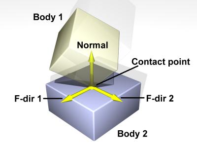
The contact joint prevents body 1 and body 2 from inter-penetrating at the contact point. It does this by only allowing the bodies to have an ``outgoing'' velocity in the direction of the contact normal. Contact joints typically have a lifetime of one time step. They are created and deleted in response to collision detection.
Contact joints can simulate friction at the contact by applying special forces in the two friction directions that are perpendicular to the normal.
When a contact joint is created, a dContact structure must be supplied. This has the following definition:
struct dContact {
  dSurfaceParameters surface;
  dContactGeom geom;
  dVector3 fdir1;
};
|
fdir1 is a "first friction direction" vector that defines a direction along which frictional force is applied. It must be of unit length and perpendicular to the contact normal (so it is typically tangential to the contact surface). It should only be defined if the dContactFDir1 flag is set in surface.mode. The "second friction direction" is a vector computed to be perpendicular to both the contact normal and fdir1.
surface is a substructure that is set by the user. Its members define the properties of the colliding surfaces. It has the following members:
| dContactMu2 | If not set, use mu for both friction directions. If set, use mu for friction direction 1, use mu2 for friction direction 2. |
| dContactFDir1 | If set, take fdir1 as friction direction 1, otherwise automatically compute friction direction 1 to be perpendicular to the contact normal (in which case its resulting orientation is unpredictable). |
| dContactBounce | If set, the contact surface is bouncy, in other words the bodies will bounce off each other. The exact amount of bouncyness is controlled by the bounce parameter. |
| dContactSoftERP | If set, the error reduction parameter of the contact normal can be set with the soft_erp parameter. This is useful to make surfaces soft. |
| dContactSoftCFM | If set, the constraint force mixing parameter of the contact normal can be set with the soft_cfm parameter. This is useful to make surfaces soft. |
| dContactMotion1 | If set, the contact surface is assumed to be moving independently of the motion of the bodies. This is kind of like a conveyor belt running over the surface. When this flag is set, motion1 defines the surface velocity in friction direction 1. |
| dContactMotion2 | The same thing as above, but for friction direction 2. |
| dContactSlip1 | Force-dependent-slip (FDS) in friction direction 1. |
| dContactSlip2 | Force-dependent-slip (FDS) in friction direction 2. |
| dContactApprox1_1 | Use the friction pyramid approximation for friction direction 1. If this is not specified then the constant-force-limit approximation is used (and mu is a force limit). |
| dContactApprox1_2 | Use the friction pyramid approximation for friction direction 2. If this is not specified then the constant-force-limit approximation is used (and mu is a force limit). |
| dContactApprox1 | Equivalent to both dContactApprox1_1 and dContactApprox1_2. |
FDS is an effect that causes the contacting surfaces to side past each other with a velocity that is proportional to the force that is being applied tangentially to that surface.
Consider a contact point where the coefficient of friction mu is infinite. Normally, if a force f is applied to the two contacting surfaces, to try and get them to slide past each other, they will not move. However, if the FDS coefficient is set to a positive value k then the surfaces will slide past each other, building up to a steady velocity of k*f relative to each other.
Note that this is quite different from normal frictional effects: the force does not cause a constant acceleration of the surfaces relative to each other - it causes a brief acceleration to achieve the steady velocity.
This is useful for modeling some situations, in particular tires. For example consider a car at rest on a road. Pushing the car in its direction of travel will cause it to start moving (i.e. the tires will start rolling). Pushing the car in the perpendicular direction will have no effect, as the tires do not roll in that direction. However - if the car is moving at a velocity v, applying a force f in the perpendicular direction will cause the tires to slip on the road with a velocity proportional to f*v (Yes, this really happens).
To model this in ODE set the tire-road contact parameters as follows: set friction direction 1 in the direction that the tire is rolling in, and set the FDS slip coefficient in friction direction 2 to k*v, where v is the tire rolling velocity and k is a tire parameter that you can chose based on experimentation.
Note that FDS is quite separate from the sticking/slipping effects of Coulomb friction - both modes can be used together at a single contact point.
An angular motor (AMotor) allows the relative angular velocities of two bodies to be controlled. The angular velocity can be controlled on up to three axes, allowing torque motors and stops to be set for rotation about those axes (see the ``Stops and motor parameters'' section below). This is mainly useful in conjunction will ball joints (which do not constrain the angular degrees of freedom at all), but it can be used in any situation where angular control is needed. To use an AMotor with a ball joint, simply attach it to the same two bodies that the ball joint is attached to.
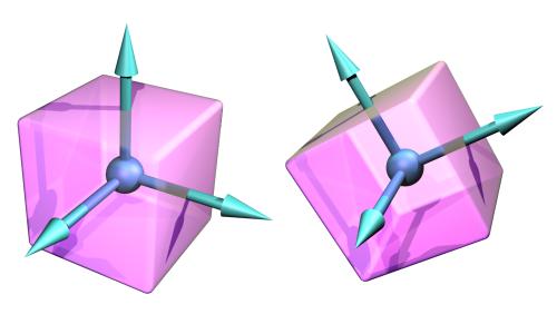
The AMotor can be used in different modes. In dAMotorUser mode, the user directly sets the axes that the AMotor controls. In dAMotorEuler mode, AMotor computes the euler angles corresponding to the relative rotation, allowing euler angle torque motors and stops to be set. An AMotor joint with euler angles looks like this:
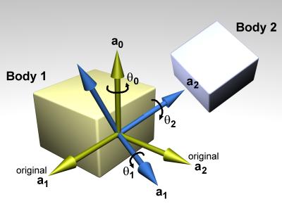
In this diagram, a0, a1 and a2 are the three axes along which angular motion is controlled. The green axes (including a0) are anchored to body 1. The blue axes (including a2) are anchored to body 2. To get the body 2 axes from the body 1 axes the following sequence of rotations is performed:
There is an important restriction when using euler angles: the theta1 angle must not be allowed to get outside the range -pi/2 ... pi/2. If this happens then the AMotor joint will become unstable (there is a singularity at +/- pi/2). Thus you must set the appropriate stops on axis number 1.
void dJointSetAMotorMode (dJointID, int mode);
int dJointGetAMotorMode (dJointID);
Set (and get) the angular motor mode. The mode parameter must be one
of the following constants:
| dAMotorUser | The AMotor axes and joint angle settings are entirely controlled by the user. This is the default mode. |
| dAMotorEuler | Euler angles are automatically computed. The axis a1 is also automatically computed. The AMotor axes must be set correctly when in this mode, as described below. When this mode is initially set the current relative orientations of the bodies will correspond to all euler angles at zero. |
void dJointSetAMotorNumAxes (dJointID, int num);
int dJointGetAMotorNumAxes (dJointID);
Set (and get) the number of angular axes that will be controlled by the
AMotor.
The argument num can range from 0 (which effectively deactivates the
joint) to 3.
This is automatically set to 3 in dAMotorEuler mode.
void dJointSetAMotorAxis (dJointID, int anum, int rel,
			  dReal x, dReal y, dReal z);
void dJointGetAMotorAxis (dJointID, int anum, dVector3 result);
int dJointGetAMotorAxisRel (dJointID, int anum);
Set (and get) the AMotor axes.
The anum argument selects the axis to change (0,1 or 2).
Each axis can have one of three ``relative orientation'' modes, selected by
rel:
The axis vector (x,y,z) is always specified in global
coordinates regardless of the setting of rel.
There are two GetAMotorAxis functions, one to return the axis and one to
return the relative mode.
For dAMotorEuler mode:
dReal dJointGetAMotorAngle (dJointID, int anum);
Return the current angle for axis anum.
In dAMotorUser mode this is simply the value that was set with
dJointSetAMotorAngle.
In dAMotorEuler mode this is the corresponding euler angle.
The joint geometry parameter setting functions should only be called after the joint has been attached to bodies, and those bodies have been correctly positioned, otherwise the joint may not be initialized correctly. If the joint is not already attached, these functions will do nothing.
For the parameter getting functions, if the system is out of alignment (i.e. there is some joint error) then the anchor/axis values will be correct with respect to body 1 only (or body 2 if you specified body 1 as zero in the dJointAttach() function).
The default anchor for all joints is (0,0,0). The default axis for all joints is (1,0,0).
When an axis is set it will be normalized to unit length. The adjusted axis is what the axis getting functions will return.
When measuring a joint angle or position, a value of zero corresponds to the initial position of the bodies relative to each other.
Note that there are no functions to set joint angles or positions (or their rates) directly, instead you must set the corresponding body positions and velocities.
When a joint is first created there is nothing to prevent it from moving through its entire range of motion. For example a hinge will be able to move through its entire angle, and a slider will slide to any length.
This range of motion can be limited by setting stops on the joint. The joint angle (or position) will be prevented from going below the low stop value, or from going above the high stop value. Note that a joint angle (or position) of zero corresponds to the initial body positions.
As well as stops, many joint types can have motors. A motor applies a torque (or force) to a joint's degree(s) of freedom to get it to pivot (or slide) at a desired speed. Motors have force limits, which means they can apply no more than a given maximum force/torque to the joint.
Motors have two parameters: a desired speed, and the maximum force that is available to reach that speed. This is a very simple model of real life motors, engines or servos. However, is it quite useful when modeling a motor (or engine or servo) that is geared down with a gearbox before being connected to the joint. Such devices are often controlled by setting a desired speed, and can only generate a maximum amount of power to achieve that speed (which corresponds to a certain amount of force available at the joint).
Motors can also be used to accurately model dry (or Coulomb) friction in joints. Simply set the desired velocity to zero and set the maximum force to some constant value - then all joint motion will be impeded by that force.
The alternative to using joint stops and motors is to simply apply forces to the affected bodies yourself. Applying motor forces is easy, and joint stops can be emulated with restraining spring forces. However applying forces directly is often not a good approach and can lead to severe stability problems if it is not done carefully.
Consider the case of applying a force to a body to achieve a desired velocity. To calculate this force you use information about the current velocity, something like this:
This has several problems. First, the parameter k must be tuned by hand. If it is too low the body will take a long time to come up to speed. If it is too high the simulation will become unstable. Second, even if k is chosen well the body will still take a few time steps to come up to speed. Third, if any other ``external'' forces are being applied to the body, the desired velocity may never even be reached (a more complicated force equation would be needed, which would have extra parameters and its own problems).
Joint motors solve all these problems: they bring the body up to speed in one time step, provided that does not take more force than is allowed. Joint motors need no extra parameters because they are actually implemented as constraints. They can effectively see one time step into the future to work out the correct force. This makes joint motors more computationally expensive than computing the forces yourself, but they are much more robust and stable, and far less time consuming to design with. This is especially true with larger rigid body systems.
Similar arguments apply to joint stops.
Here are the functions that set stop and motor parameters (as well as other kinds of parameters) on a joint:
void dJointSetHingeParam (dJointID, int parameter, dReal value);
void dJointSetSliderParam (dJointID, int parameter, dReal value);
void dJointSetHinge2Param (dJointID, int parameter, dReal value);
void dJointSetAMotorParam (dJointID, int parameter, dReal value);
dReal dJointGetHingeParam (dJointID, int parameter);
dReal dJointGetSliderParam (dJointID, int parameter);
dReal dJointGetHinge2Param (dJointID, int parameter);
dReal dJointGetAMotorParam (dJointID, int parameter);
Set/get limit/motor parameters for each joint type.
The parameter numbers are:
| dParamLoStop | Low stop angle or position. Setting this to -dInfinity (the default value) turns off the low stop. For rotational joints, this stop must be greater than -Pi to be effective. |
| dParamHiStop | High stop angle or position. Setting this to dInfinity (the default value) turns off the high stop. For rotational joints, this stop must be less than Pi to be effective. If the high stop is less than the low stop then both stops will be ineffective. |
| dParamVel | Desired motor velocity (this will be an angular or linear velocity). |
| dParamFMax | The maximum force or torque that the motor will use to achieve the desired velocity. This must always be greater than or equal to zero. Setting this to zero (the default value) turns off the motor. |
| dParamFudgeFactor | The current joint stop/motor implementation has a small problem: when the joint is at one stop and the motor is set to move it away from the stop, too much force may be applied for one time step, causing a ``jumping'' motion. This fudge factor is used to scale this excess force. It should have a value between zero and one (the default value). If the jumping motion is too visible in a joint, the value can be reduced. Making this value too small can prevent the motor from being able to move the joint away from a stop. |
| dParamBounce | The bouncyness of the stops. This is a restitution parameter in the range 0..1. 0 means the stops are not bouncy at all, 1 means maximum bouncyness. |
| dParamCFM | The constraint force mixing (CFM) value used when not at a stop. |
| dParamStopERP | The error reduction parameter (ERP) used by the stops. |
| dParamStopCFM | The constraint force mixing (CFM) value used by the stops. Together with the ERP value this can be used to get spongy or soft stops. Note that this is intended for unpowered joints, it does not really work as expected when a powered joint reaches its limit. |
| dParamSuspensionERP | Suspension error reduction parameter (ERP). Currently this is only implemented on the hinge-2 joint. |
| dParamSuspensionCFM | Suspension constraint force mixing (CFM) value. Currently this is only implemented on the hinge-2 joint. |
If a particular parameter is not implemented by a given joint, setting it will have no effect.
These parameter names can be optionally followed by a digit (2 or 3) to indicate the second or third set of parameters, e.g. for the second axis in a hinge-2 joint, or the third axis in an AMotor joint. A constant dParamGroup is also defined such that:
ODE's dWorldStep function currently uses a "big matrix" method to step the system. For some large systems this can be slow and can require a lot of memory. The StepFast1 algorithm provides an alternative way to step the system, that sacrifices some accuracy for a big gain in speed and memory. To use it, you simply call dWorldStepFast1 instead of dWorldStep.
The chart below illustrates this speed advantage over the standard dWorldStep algorithm:
The graph relates the number of Degrees Of Freedom (DOFs) removed from a system to the running time of the step. You may be able to tell that the dWorldStep algorithm's running time is proportional to the cube of the number of DOF's removed. The StepFast1 algorithm, however, is roughly linear. So as islands increase in size (for example, when there is a large pile-up of cars, a pile of "ragdoll corpses", or a wall of bricks) the StepFast1 algorithm scales better than dWorldStep. All this means that your application is more likely to keep a steady framerate, even in the worst case scenario.
The graph of DOFs removed to memory looks quite similar.
dWorldStep requires memory proportional only to the square of the number of DOF's removed. StepFast1, though, is still linear, but it has nothing to do with the number of iterations per step. So this means the dreaded "There was a big pile-up and ODE crashed without an error message" problems (usually stack overflows) won't happen with StepFast1. Or at least that you'll be rendering at a minute per frame or slower before they do.
As shown above, StepFast1 is quite good when it comes to speed and memory usage. All this power doesn't come for free, though; all optimizations are a trade-off of one kind or another. I've already mentioned that StepFast1 trades off accuracy for it's speed and memory advantages. You actually get to choose just how much accuracy you give away though, at the cost of speed, by adjusting the number of iterations per step. Though you may never reach the accuracy of dWorldStep (or you may surpass it, depending on the type of inaccuracy), you can be almost certain that a larger number of iterations will give you more accurate results (more slowly). So StepFast1 can be used in a good variety of situations.
The general answer to this question then, is: use StepFast1 when you don't mind having a few more parameters to play with to get the system stable, and you want to take advantage of it's speed or memory advantages. If you find yourself running into situations in your simulation where large numbers of bodies come in contact, and dWorldStep becomes too slow, try switching to StepFast1. Many systems will work just fine with nothing more than changing the dWorldStep function call to dWorldStepFast1. Others will require a little tweaking to get them to work well with StepFast1, usually in the masses of the bodies. When a joint connects two bodies with a large mass ratio (i.e. one body has several times the mass of the other body) StepFast1 may have trouble solving it.
Another prospect for StepFast1 is designing for it from the ground up. If you know you are going to build large worlds with many physically based objects in them, then go ahead and plan to use StepFast1. Noting the mass ratio problem above, you might want to consider making the mass of every body in your system equal to 1.0. Or in a very small range, for example between 0.5 and 1.5. Most of the other suggestions for speed and stability apply to StepFast1, except that the object is no longer to remove as many joints as possible from the equation. It can likely be shown that you will get a better performance to stability ratio by spreading out mass among several bodies connected by fixed joints rather than trying to implement it as one massive body, especially if that one massive body means you have to switch back to dWorldStep to keep things stable.
A final prospect for StepFast1 is to use it only when you need to. Since StepFast1 uses the body and world structures in exactly the same way as dWorldStep, you can actually switch back and forth between the two solvers at will. A good heuristic for when to make this switch is to simply count contact joints while you are running the collision detection. Since collision detection is normally called before the step, using this method will ensure that the large island that would slow you down is never sent to the dWorldStep solver (as opposed to waiting until after you've already taken a step at 1 fps...). The only better solution would be a hybrid island creation function, that sends small islands to dWorldStep, and large islands to dWorldStepFast1. This may make it in the source at some point in the future.
Though there are several specific situations when it as advisable not to use StepFast1, I believe they can all be summed up in a single statement: Don't use StepFast1 when accuracy is more important than speed or memory to you. You may still want to evaluate it in this case and see if the inaccuracies are even noticeable, perhaps with a relatively large number of iterations (20+).
For any interested parties out there, here's a quick rundown of how the StepFast1 algorithm works. The general problem that ODE tries to solve is a system of linear (in)equalities in (m = constraints) unknowns, where one constraint constrains 1 Degree of Freedom in one joint. For large islands of bodies with many joints between them, this can take a rather large O(m2) array, which takes O(m3) time to solve. StepFast1 completely avoids creating the large matrix by making an assumption: at relatively small timesteps, the effect of any given joint is so localized that it can be calculated without respect to any other joint in the system, and any conflicting joints will cancel each other out before the body actually moves. So StepFast1 uses the same solution method (LCP) to solve the same problem, only localized to a single joint (where m <= 6). It gets away with this by sub-dividing the timestep and repeating the process over really small timesteps (i = maxiterations) times. So the running time of StepFast1 is "roughly" O(m i). It's really closer to O(j i (m/j)3) = O(m i (m/j)2), where j = joints, but (m/j) is never > 6, so (m/j)2 is factored out as a constant.
Several experimental functions have been added to ODE as part of the StepFast1 flow of code, at least until they are validated. Most have to do with the automatic disabling and enabling of bodies as yet another bit of optimization. Here's the general idea:
void dWorldSetAutoEnableDepthSF1(dWorldID, int autoEnableDepth);
int dWorldGetAutoEnableDepthSF1(dWorldID);
Set and get the AutoEnableDepth parameter used by the StepFast1 algorithm.
void dBodySetAutoDisableThresholdSF1(dBodyID, dReal autoDisableThreshold);
dReal dBodyGetAutoDisableThresholdSF1(dBodyID);
Set and get the per-body AutoDisableThreshold parameter used by the
StepFast1 algorithm.
void dBodySetAutoDisableStepsSF1(dBodyID, int AutoDisableSteps);
int dBodyGetAutoDisableStepsSF1(dBodyID);
Set and get the per-body AutoDisableSteps parameter used by the StepFast1
algorithm.
void dBodySetAutoDisableSF1(dBodyID, int doAutoDisable);
int dBodyGetAutoDisableSF1(dBodyID);
Set and get the per-body AutoDisable flag used by the StepFast1 algorithm.
If doAutoDisable is nonzero, auto-disabling is enabled.
If doAutoDisable is zero, auto-disabling is disabled.
Rigid body orientations are represented with quaternions. A quaternion is four numbers [cos(theta/2) sin(theta/2)*u] where theta is a rotation angle and `u' is a unit length rotation axis.
Every rigid body also has a 3x3 rotation matrix that is derived from the quaternion. The rotation matrix and the quaternion always match.
Some information about quaternions:
The following are utility functions for dealing with rotation matrices and quaternions.
void dRSetIdentity (dMatrix3 R);
Set R to the identity matrix (i.e. no rotation).
void dQSetIdentity (dQuaternion q);
Set q to the identity rotation (i.e. no rotation).
void dQMultiply0 (dQuaternion qa,
                  const dQuaternion qb, const dQuaternion qc);
void dQMultiply1 (dQuaternion qa,
                  const dQuaternion qb, const dQuaternion qc);
void dQMultiply2 (dQuaternion qa,
                  const dQuaternion qb, const dQuaternion qc);
void dQMultiply3 (dQuaternion qa,
                  const dQuaternion qb, const dQuaternion qc);
Set qa = qb*qc.
This is that same as qa = rotation qc followed by rotation
qb.
The 0/1/2 versions are analogous to the multiply functions, i.e. 1 uses the
inverse of qb, and 2 uses the inverse of qc.
Option 3 uses the inverse of both.
void dQtoR (const dQuaternion q, dMatrix3 R);
Convert quaternion q to rotation matrix R.
void dRtoQ (const dMatrix3 R, dQuaternion q);
Convert rotation matrix R to quaternion q.
The mass parameters of a rigid body are described by a dMass structure:
typedef struct dMass {
  dReal mass;   // total mass of the rigid body
  dVector4 c;   // center of gravity position in body frame (x,y,z)
  dMatrix3 I;   // 3x3 inertia tensor in body frame, about POR
} dMass;
|
The following functions operate on this structure:
void dMassSetZero (dMass *);
Set all the mass parameters to zero.
void dMassSetSphere (dMass *, dReal density, dReal radius);
void dMassSetSphereTotal (dMass *, dReal total_mass, dReal radius);
Set the mass parameters to represent a sphere of the given radius and
density, with the center of mass at (0,0,0) relative to the body. The
first function accepts the density of the sphere, the second accepts
the total mass of the sphere.
void dMassSetCappedCylinder (dMass *, dReal density, int direction,
                             dReal radius, dReal length);
void dMassSetCappedCylinderTotal (dMass *, dReal total_mass, int direction,
                             dReal radius, dReal length);
Set the mass parameters to represent a capped cylinder of the given parameters
and density, with the center of mass at (0,0,0) relative to the body.
The radius of the cylinder (and the spherical cap) is radius.
The length of the cylinder (not counting the spherical cap) is length.
The cylinder's long axis is oriented along the body's x, y or z axis according
to the value of direction (1=x, 2=y, 3=z). The
first function accepts the density of the object, the second accepts
its total mass.
void dMassSetCylinder (dMass *, dReal density, int direction,
		       dReal radius, dReal length);
void dMassSetCylinderTotal (dMass *, dReal total_mass, int direction,
		       dReal radius, dReal length);
Set the mass parameters to represent a flat-ended cylinder of the given
parameters and density, with the center of mass at (0,0,0) relative to the
body.
The radius of the cylinder is radius.
The length of the cylinder is length.
The cylinder's long axis is oriented along the body's x, y or z axis according
to the value of direction (1=x, 2=y, 3=z). The
first function accepts the density of the object, the second accepts
its total mass.
void dMassSetBox (dMass *, dReal density,
                  dReal lx, dReal ly, dReal lz);
void dMassSetBoxTotal (dMass *, dReal total_mass,
                  dReal lx, dReal ly, dReal lz);
Set the mass parameters to represent a box of the given dimensions
and density, with the center of mass at (0,0,0) relative to the body.
The side lengths of the box along the x, y and z axes are lx, ly
and lz. The
first function accepts the density of the object, the second accepts
its total mass.
void dMassAdd (dMass *a, const dMass *b);
Add the mass b to the mass a.
[There are quite a lot of these, but they're not standardized enough to document yet].
[Document these later].
ODE has two main components: a dynamics simulation engine and a collision detection engine. The collision engine is given information about the shape of each body. At each time step it figures out which bodies touch each other and passes the resulting contact point information to the user. The user in turn creates contact joints between bodies.
Using ODE's collision detection is optional - an alternative collision detection system can be used as long as it can supply the right kinds of contact information.
If two bodies touch, or if a body touches a static feature in its environment, the contact is represented by one or more "contact points". Each contact point has a corresponding dContactGeom structure:
struct dContactGeom {
  dVector3 pos;       // contact position
  dVector3 normal;    // normal vector
  dReal depth;        // penetration depth
  dGeomID g1,g2;      // the colliding geoms
};
|
depth is the depth to which the two bodies inter-penetrate each other. If the depth is zero then the two bodies have a grazing contact, i.e. they "only just" touch. However, this is rare - the simulation is not perfectly accurate and will often step the bodies too far so that the depth is nonzero.
normal is a unit length vector that is, generally speaking, perpendicular to the contact surface.
g1 and g2 are the geometry objects that collided.
The convention is that if body 1 is moved along the normal vector by a distance depth (or equivalently if body 2 is moved the same distance in the opposite direction) then the contact depth will be reduced to zero. This means that the normal vector points "in" to body 1.
In real life, contact between two bodies is a complex thing. Representing contacts by contact points is only an approximation. Contact "patches" or "surfaces" might be more physically accurate, but representing these things in high speed simulation software is a challenge.
Each extra contact point added to the simulation will slow it down some more, so sometimes we are forced to ignore contact points in the interests of speed. For example, when two boxes collide many contact points may be needed to properly represent the geometry of the situation, but we may choose to keep only the best three. Thus we are piling approximation on top of approximation.
Geometry objects (or ``geoms'' for short) are the fundamental objects in the collision system. A geom can represents a single rigid shape (such as a sphere or box), or it can represents a group of other geoms - this is a special kind of geom called a ``space''.
Any geom can be collided against any other geom to yield zero or more contact points. Spaces have the extra capability of being able to collide their contained geoms together to yield internal contact points.
Geoms can be placeable or non-placeable. A placeable geom has a position vector and a 3*3 rotation matrix, just like a rigid body, that can be changed during the simulation. A non-placeable geom does not have this capability - for example, it may represent some static feature of the environment that can not be moved. Spaces are non-placeable geoms, because each contained geom may have its own position and orientation but it does not make sense for the space itself to have a position and orientation.
To use the collision engine in a rigid body simulation, placeable geoms are associated with rigid body objects. This allows the collision engine to get the position and orientation of the geoms from the bodies. Note that geoms are distinct from rigid bodies in that a geom has geometrical properties (size, shape, position and orientation) but no dynamical properties (such as velocity or mass). A body and a geom together represent all the properties of the simulated object.
Every geom is an instance of a class, such as sphere, plane, or box. There are a number of built-in classes, described below, and you can define your own classes as well.
The point of reference of a placeable geoms is the point that is controlled by its position vector. The point of reference for the standard classes usually corresponds to the geom's center of mass. This feature allows the standard classes to be easily connected to dynamics bodies. If other points of reference are required, a transformation object can be used to encapsulate a geom.
The concepts and functions that apply to all geoms will be described below, followed by the various geometry classes and the functions that manipulate them.
A space is a non-placeable geom that can contain other geoms. It is similar to the rigid body concept of the ``world'', except that it applies to collision instead of dynamics.
Space objects exist to make collision detection go faster. Without spaces, you might generate contacts in your simulation by calling dCollide() to get contact points for every single pair of geoms. For N geoms this is O(N2) tests, which is too computationally expensive if your environment has many objects.
A better approach is to insert the geoms into a space and call dSpaceCollide(). The space will then perform collision culling, which means that it will quickly identify which pairs of geoms are potentially intersecting. Those pairs will be passed to a callback function, which can in turn call dCollide() on them. This saves a lot of time that would have been spent in useless dCollide() tests, because the number of pairs passed to the callback function will be a small fraction of every possible object-object pair.
Spaces can contain other spaces. This is useful for dividing a collision environment into several hierarchies to further optimize collision detection speed. This will be described in more detail below.
The following functions can be applied to any geom.
When a space is destroyed, if its cleanup mode is 1 (the default) then all the geoms in that space are automatically destroyed as well.
void dGeomSetData (dGeomID, void *);
void *dGeomGetData (dGeomID);
These functions set and get the user-defined data pointer stored in the
geom.
void dGeomSetBody (dGeomID, dBodyID);
dBodyID dGeomGetBody (dGeomID);
These functions set and get the body associated with a placeable geom.
Setting a body on a geom automatically combines the position vector
and rotation matrix of the body and geom, so that setting the position
or orientation of one will set the value for both objects.
Setting a body ID of zero gives the geom its own position and rotation, independent from any body. If the geom was previously connected to a body then its new independent position/rotation is set to the current position/rotation of the body.
Calling these functions on a non-placeable geom results in a runtime error in the debug build of ODE.
void dGeomSetPosition (dGeomID, dReal x, dReal y, dReal z);
void dGeomSetRotation (dGeomID, const dMatrix3 R);
void dGeomSetQuaternion (dGeomID, const dQuaternion);
Set the position vector, rotation matrix or quaternion of a placeable geom.
These functions are analogous to dBodySetPosition(),
dBodySetRotation() and dBodySetQuaternion().
If the geom is attached to a body, the body's position / rotation / quaternion
will also be changed.
Calling these functions on a non-placeable geom results in a runtime error in the debug build of ODE.
const dReal * dGeomGetPosition (dGeomID);
const dReal * dGeomGetRotation (dGeomID);
void dGeomGetQuaternion (dGeomID, dQuaternion result);
The first two return pointers to the geom's position vector and rotation matrix.
The returned values are pointers to internal data structures, so the vectors
are valid until any changes are made to the geom.
If the geom is attached to a body, the body's position / rotation
pointers will be returned, i.e. the result will be identical to calling
dBodyGetPosition() or dBodyGetRotation().
dGeomGetQuaternion() copies the geom's quaternion into the space provided. If the geom is attached to a body, the body's quaternion will be returned, i.e. the resulting quaternion will be the same as the result of calling dBodyGetQuaternion().
Calling these functions on a non-placeable geom results in a runtime error in the debug build of ODE.
This function may return a pre-computed cached bounding box, if it can determine that the geom has not moved since the last time the bounding box was computed.
int dGeomIsSpace (dGeomID);
Return 1 if the given geom is a space, or 0 if not.
| dSphereClass | Sphere |
| dBoxClass | Box |
| dCCylinderClass | Capped cylinder |
| dCylinderClass | Regular flat-ended cylinder |
| dPlaneClass | Infinite plane (non-placeable) |
| dGeomTransformClass | Geometry transform |
| dRayClass | Ray |
| dTriMeshClass | Triangle mesh |
| dSimpleSpaceClass | Simple space |
| dHashSpaceClass | Hash table based space |
User defined classes will return their own numbers.
void dGeomSetCategoryBits (dGeomID, unsigned long bits);
void dGeomSetCollideBits (dGeomID, unsigned long bits);
unsigned long dGeomGetCategoryBits (dGeomID);
unsigned long dGeomGetCollideBits (dGeomID);
Set and get the ``category'' and ``collide'' bitfields for the given geom.
These bitfields are use by spaces to govern which geoms will interact
with each other.
The bit fields are guaranteed to be at least 32 bits wide.
The default category and collide values for newly created geoms have
all bits set.
void dGeomEnable (dGeomID);
void dGeomDisable (dGeomID);
int dGeomIsEnabled (dGeomID);
Enable and disable a geom.
Disabled geoms are completely ignored by dSpaceCollide() and
dSpaceCollide2(), although they can still be members of a space.
dGeomIsEnabled() returns 1 if a geom is enabled or 0 if it is disabled. New geoms are created in the enabled state.
A collision detection ``world'' is created by making a space and then adding geoms to that space. At every time step we want to generate a list of contacts for all the geoms that intersect each other. Three functions are used to do this:
The collision system has been designed to give the user maximum flexibility to decide which objects will be tested against each other. This is why are there are three collision functions instead of, for example, one function that just generates all the contact points.
Spaces may contain other spaces. These sub-spaces will typically represent a collection of geoms (or other spaces) that are located near each other. This is useful for gaining extra collision performance by dividing the collision world into hierarchies. Here is an example of where this is useful:
Suppose you have two cars driving over some terrain. Each car is made up of many geoms. If all these geoms were inserted into the same space, the collision computation time between the two cars would always be proportional to the total number of geoms (or even to the square of this number, depending on which space type is used).To speed up collision a separate space is created to represent each car. The car geoms are inserted into the car-spaces, and the car-spaces are inserted into the top level space. At each time step dSpaceCollide() is called for the top level space. This will do a single intersection test between the car-spaces (actually between their bounding boxes) and call the callback if they touch. The callback can then test the geoms in the car-spaces against each other using dSpaceCollide2(). If the cars are not near each other then the callback is not called and no time is wasted performing unnecessary tests.
If space hierarchies are being used then the callback function may be called recursively, e.g. if dSpaceCollide() calls the callback which in turn calls dSpaceCollide() with the same callback function. In this case the user must make sure that the callback function is properly reentrant.
Here is a sample callback function that traverses through all spaces and sub-spaces, generating all possible contact points for all intersecting geoms:
  void nearCallback (void *data, dGeomID o1, dGeomID o2)
  {
    if (dGeomIsSpace (o1) || dGeomIsSpace (o2)) {
      // colliding a space with something
      dSpaceCollide2 (o1,o2,data,&nearCallback);
      // collide all geoms internal to the space(s)
      if (dGeomIsSpace (o1)) dSpaceCollide (o1,data,&nearCallback);
      if (dGeomIsSpace (o2)) dSpaceCollide (o2,data,&nearCallback);
    }
    else {
      // colliding two non-space geoms, so generate contact
      // points between o1 and o2
      int num_contact = dCollide (o1,o2,max_contacts,contact_array,skip);
      // add these contact points to the simulation
      ...
    }
  }

  ...

  // collide all objects together
  dSpaceCollide (top_level_space,0,&nearCallback);
|
A space callback function is not allowed to modify a space while that space is being processed with dSpaceCollide() or dSpaceCollide2(). For example, you can not add or remove geoms from a space, and you can not reposition the geoms within a space. Doing so will trigger a runtime error in the debug build of ODE.
Each geom has a ``category'' and ``collide'' bitfield that can be used to assist the space algorithms in determining which geoms should interact and which should not. Use of this feature is optional - by default geoms are considered to be capable of colliding with any other geom.
Each bit position in the bitfield represents a different category of object. The actual meaning of these categories (if any) is user defined. The category bitfield indicates which categories a geom is a member of. The collide bitfield indicates which categories the geom will collide with during collision detection.
A pair of geoms will be considered by dSpaceCollide() and dSpaceCollide2() for passing to the callback only if one of them has a collide bit set that corresponds to a category bit in the other. The exact test is as follows:
  // test if geom o1 and geom o2 can collide
  cat1 = dGeomGetCategoryBits (o1);
  cat2 = dGeomGetCategoryBits (o2);
  col1 = dGeomGetCollideBits (o1);
  col2 = dGeomGetCollideBits (o2);
  if ((cat1 & col2) || (cat2 & col1)) {
    // call the callback with o1 and o2
  }
  else {
    // do nothing, o1 and o2 do not collide
  }
|
Note that only dSpaceCollide() and dSpaceCollide2() use these bitfields, they are ignored by dCollide().
Typically a geom will belong only to a single category, so only one bit will be set in the category bitfield. The bitfields are guaranteed to be at least 32 bits wide, so the user is able to specify an arbitrary pattern of interactions for up to 32 objects. If there are more than 32 objects then some of them will obviously have to have the same category.
Sometimes the category field will contain multiple bits set, e.g. if the geom is a space them you may want to set the category to the union of all the geom categories that are contained.
Design note: Why don't we just have a single category bitfield and use the test (cat1 & cat2) ? This is simpler, but a single field requires more bits to represent some patterns of interaction. For example, if 32 geoms have an interaction pattern that is a 5 dimensional hypercube, 80 bit are required in the simpler scheme. The simpler scheme also makes it harder to determine what the categories should be for some situations.
flags specifies how contacts should be generated if the geoms touch. The lower 16 bits of flags is an integer that specifies the maximum number of contact points to generate. Note that if this number is zero, this function just pretends that it is one - in other words you can not ask for zero contacts. All other bits in flags must be zero. In the future the other bits may be used to select from different contact generation strategies.
contact points to an array of dContactGeom structures. The array must be able to hold at least the maximum number of contacts. These dContactGeom structures may be embedded within larger structures in the array - the skip parameter is the byte offset from one dContactGeom to the next in the array. If skip is sizeof(dContactGeom) then contact points to a normal (C-style) array. It is an error for skip to be smaller than sizeof(dContactGeom).
If the geoms intersect, this function returns the number of contact points generated (and updates the contact array), otherwise it returns 0 (and the contact array is not touched).
If a space is passed as o1 or o2 then this function will collide all objects contained in o1 with all objects contained in o2, and return the resulting contact points. This method for colliding spaces with geoms (or spaces with spaces) provides no user control over the individual collisions. To get that control, use dSpaceCollide() or dSpaceCollide2() instead.
If o1 and o2 are the same geom then this function will do nothing and return 0. Technically speaking an object intersects with itself, but it is not useful to find contact points in this case.
This function does not care if o1 and o2 are in the same space or not (or indeed if they are in any space at all).
void dSpaceCollide (dSpaceID space,
                    void *data, dNearCallback *callback);
This determines which pairs of geoms in a space may potentially intersect,
and calls the callback function with each candidate pair.
The callback function is of type dNearCallback, which is defined as:
The data argument is passed from dSpaceCollide() directly
to the callback function. Its meaning is user defined.
The o1 and o2 arguments are the geoms that may be near
each other.
typedef void dNearCallback (void *data, dGeomID o1, dGeomID o2);
The callback function can call dCollide() on o1 and o2 to generate contact points between each pair. Then these contact points may be added to the simulation as contact joints. The user's callback function can of course chose not to call dCollide() for any pair, e.g. if the user decides that those pairs should not interact.
Other spaces that are contained within the colliding space are not treated specially, i.e. they are not recursed into. The callback function may be passed these contained spaces as one or both geom arguments.
dSpaceCollide() is guaranteed to pass all intersecting geom pairs to the callback function, but it may also make mistakes and pass non-intersecting pairs. The number of mistaken calls depends on the internal algorithms used by the space. Thus you should not expect that dCollide() will return contacts for every pair passed to the callback.
void dSpaceCollide2 (dGeomID o1, dGeomID o2,
                     void *data, dNearCallback *callback);
This function is similar to dSpaceCollide(), except that it is passed two geoms (or spaces) as arguments. It calls the callback for all potentially intersecting pairs that contain one geom from o1 and one geom from o2.
The exact behavior depends on the types of o1 and o2:
There are several kinds of spaces. Each kind uses different internal data structures to store the geoms, and different algorithms to perform the collision culling:
Here are the functions used for spaces:
dSpaceID dSimpleSpaceCreate (dSpaceID space);
dSpaceID dHashSpaceCreate (dSpaceID space);
Create a space, either of the simple or multi-resolution hash table kind.
If space is nonzero, insert the new space into that space.
void dSpaceDestroy (dSpaceID);
This destroys a space. It functions exactly like dGeomDestroy()
except that it takes a dSpaceID argument.
When a space is destroyed, if its cleanup mode is 1 (the default) then
all the geoms in that space are automatically destroyed as well.
void dSpaceSetCleanup (dSpaceID space, int mode);
int dSpaceGetCleanup (dSpaceID space);
Set and get the clean-up mode of the space.
If the clean-up mode is 1, then the contained geoms will be destroyed when
the space is destroyed. If the clean-up mode is 0 this does not happen.
The default clean-up mode for new spaces is 1.
void dSpaceRemove (dSpaceID, dGeomID);
Remove a geom from a space.
This does nothing if the geom is not actually in the space.
This function is called automatically by dGeomDestroy() if the
geom is in a space.
int dSpaceGetNumGeoms (dSpaceID);
Return the number of geoms contained within a space.
If any change is made to the space (including adding and deleting geoms) then no guarantee can be made about how the index number of any particular geom will change. Thus no space changes should be made while enumerating the geoms.
This function is guaranteed to be fastest when the geoms are accessed in the order 0,1,2,etc. Other nonsequential orders may result in slower access, depending on the internal implementation.
void dGeomSphereSetRadius (dGeomID sphere, dReal radius);
Set the radius of the given sphere.
dReal dGeomSphereGetRadius (dGeomID sphere);
Return the radius of the given sphere.
A capped cylinder is like a normal cylinder except it has half-sphere caps at its ends. This feature makes the internal collision detection code particularly fast and accurate. The cylinder's length, not counting the caps, is given by length. The cylinder is aligned along the geom's local Z axis. The radius of the caps, and of the cylinder itself, is given by radius.
A ray is different from all the other geom classes in that it does not represent a solid object. It is an infinitely thin line that starts from the geom's position and extends in the direction of the geom's local Z-axis.
Calling dCollide() between a ray and another geom will result in at most one contact point. Rays have their own conventions for the contact information in the dContactGeom structure (thus it is not useful to create contact joints from this information):
Rays are useful for things like visibility testing, detemining the path of projectiles or light rays, and for object placement.
void dGeomRaySetLength (dGeomID ray, dReal length);
Set the length of the given ray.
dReal dGeomRayGetLength (dGeomID ray);
Get the length of the given ray.
Geometry groups are deprecated, their functionality is now available through spaces. The geometry group functions are still available but they will be removed in some future version of ODE.
The geometry group functions are equivalent to the following space functions:
It used to be the case that if the user wanted the geoms inside a geometry group to self-intersect then the geoms would have to be inserted into a separate space and dSpaceCollide() called on that. This is no longer the case: dSpaceCollide() can be called on the geometry group directly (as it is now the same as a regular space).
A geometry transform `T' is a geom that encapsulates another geom `E', allowing E to be positioned and rotated arbitrarily with respect to its point of reference.
Most placeable geoms (like the sphere and box) have their point of reference corresponding to their center of mass, allowing them to be easily connected to dynamics objects. Transform objects give you more flexibility - for example, you can offset the center of a sphere, or rotate a cylinder so that its axis is something other than the default.
T mimics the object E that it encapsulates: T is inserted into a space and attached to a body as though it was E. E itself must not be inserted into a space or attached to a body. E's position and rotation are set to constant values that say how it is transformed relative to T. If E's position and rotation are left at their default values, T will behave exactly like E would have if you had used it directly.
If g has its clean-up mode turned on, and it already encapsulates an object, the old object will be destroyed before it is replaced with the new one.
dGeomID dGeomTransformGetGeom (dGeomID g);
Get the geom that the geometry transform g encapsulates.
void dGeomTransformSetCleanup (dGeomID g, int mode);
int dGeomTransformGetCleanup (dGeomID g);
Set and get the clean-up mode of geometry transform g.
If the clean-up mode is 1, then the encapsulated object will be destroyed
when the geometry transform is destroyed.
If the clean-up mode is 0 this does not happen.
The default clean-up mode is 0.
void dGeomTransformSetInfo (dGeomID g, int mode);
int dGeomTransformGetInfo (dGeomID g);
Set and get the "information" mode of geometry transform g.
The mode can be 0 or 1. The default mode is 0.
With mode 0, when a transform object is collided with another object (using dCollide (tx_geom,other_geom,...)), the g1 field of the dContactGeom structure is set to the geom that is encapsulated by the transform object. This value of g1 allows the caller to interrogate the type of the geom that is transformed, but it does not allow the caller to determine the position in global coordinates or the associated body, as both of these properties are used differently for encapsulated geoms.
With mode 1, the g1 field of the dContactGeom structure is set to the transform object itself. This makes the object appear just like any other kind of geom, as dGeomGetBody() will return the attached body, and dGeomGetPosition() will return the global position. To get the actual type of the encapsulated geom in this case, dGeomTransformGetGeom() must be used.
ODE's geometry classes are implemented internally as C++ classes. If you want to define your own geometry classes you can do this in two ways:
Every user defined geometry class has a unique integer number. A new geometry class (call it `X') must provide the following to ODE:
typedef int dColliderFn (dGeomID o1, dGeomID o2, int flags,
                         dContactGeom *contact, int skip);
|
typedef dColliderFn * dGetColliderFnFn (int num); |
This function is called infrequently - the return values are cached and reused.
typedef void dGetAABBFn (dGeomID g, dReal aabb[6]); |
typedef void dGeomDtorFn (dGeomID o); |
typedef int dAABBTestFn (dGeomID o1, dGeomID o2, dReal aabb2[6]); |
This is useful, for example, for large terrains. Terrains typically have very large AABBs, which are not very useful to test intersections with other objects. This function can test another object's AABB against the terrain without going to the computational trouble of calling the specific collision function. This has an especially big savings when testing against GeomGroup objects.
Here are the functions used to manage custom classes:
Here is the definition of the dGeomClass structure:
struct dGeomClass {
  int bytes;                  // bytes of custom data needed
  dGetColliderFnFn *collider; // collider function
  dGetAABBFn *aabb;           // bounding box function
  dAABBTestFn *aabb_test;     // aabb tester, can be 0 for none
  dGeomDtorFn *dtor;          // destructor, can be 0 for none
};
|
dGeomID dCreateGeom (int classnum);
Create a geom of the given class number.
The custom data block will initially be set to 0.
This object can be added to a space using dSpaceAdd().
When you implement a new class you will usually write a function that does the following:
Consider the following objects:
No extra functions are needed to manage composite objects: simply create each component geom and attach it to the same body. To move and rotate the separate geoms with respect to each other in the same object, geometry transforms can be used to encapsulate them. That's all there is to it!
However there is one caveat: You should never create a composite object that will result in collision points being generated very close together. For example, consider a table that is made up of a box for the top and four boxes for the legs. If the legs are flush with the top, and the table is lying on the ground on its side, then the contact points generated for the boxes may coincide where the legs join to the top. ODE does not currently optimize away coincident contact points, so this situation can lead to numerical errors and strange behavior.
In this example the table geometry should be adjusted so that the legs are not flush with the sides, making it much more unlikely that coincident contact points will be generated. In general, avoid having different contact surfaces that overlap, or that line up along their edges.
Often the collision world will contain many objects that are part of the static environment, that are not associated with rigid bodies. ODE's collision detection is optimized to detect geoms that do not move and to precompute as much information as possible about these objects to save time. For example, bounding boxes and internal collision data structures are precomputed.
Using ODE's collision detection is optional - an alternative collision library can be used as long as it can supply dContactGeom structures to initialize contact joints.
The dynamics core of ODE is mostly independent of the collision library that is used, except for four points:
void dGeomMoved (dGeomID); |
This function is called by the dynamics code whenever a body moves: it indicates that the geometry object associated with the body is now in a new position.
dGeomID dGeomGetBodyNext (dGeomID); |
This function is called by the dynamics code to traverse the list of geoms that are associated with each body. Given a geom attached to a body, it returns the next geom attached to that body, or 0 if there are no more geoms.
void dGeomSetBody (dGeomID, dBodyID); |
This function is called in the body destructor code (with the second argument set to 0) to remove all references from the geom to the body.
[just notes for now]
What factors does execution speed depend on? Each joint removes a number of degrees of freedom (DOFs) from the system. For example the ball and socket removes three, and the hinge removes five. For each separate group of bodies connected by joints, where:
ODE currently relies on factorization of a ``system'' matrix that has one row/column for each DOF removed (this is where the O(m23) comes from). In a 10 body chain that uses ball and socket joints, roughly 30-40% of the time is spent filling in this matrix, and 30-40% of the time is spent factorizing it.
Thus, to speed up your simulation you might consider:
Increasing the global CFM will make the system more numerically robust and less susceptable to stability problems. It will also make the system look more ``spongy'', so a tradeoff has to be found.
Redundant constraints (two or more constraints that ``try and do the same job'') will fight each other and cause stability problems. The numerical cause of this problem is singularity in the system matrix. One example of this is if two contacts joints connect the same pair of bodies at the same point. Another example is if a virtual hinge joint is created between two bodies by connecting them with two ball joints, spaced apart along the hinge axis (this is bad because the two ball joints try to remove six degrees of freedom from the system, but a real hinge joint would only remove five).
Redundant constraints fight each other and generate strange forces in the system that can swamp the normal forces. For example, an affected body might fly around as though it has a life of its own, with complete disregard for gravity.
This chapter has some common questions and their answers. For further information, you can check out the ODE Wiki, a community-supported website.
Use dJointAttach with arguments (body,0) or (0,body).
No. ODE is a computational engine, and is completely independent of any graphics library. However the examples that come with ODE use OpenGL, and most interesting uses of ODE will need some graphics library to make the simulation visible to the user. But that's your problem.
Sometimes when rigid bodies collide without restitution, they appear to inter-penetrate slightly and then get pushed apart so that they only just touch. The problem gets worse as the time step gets larger. What is going on?
The contact joint constraint is only applied after the collision is detected. If a fixed time step is being used, it is likely that the bodies have already penetrated when this happens. The error reduction mechanism will push the bodies apart, but this can take a few time steps (depending on the value of the ERP parameter).
This penetration and pushing apart sometimes makes the bodies look like they are bouncing, although it is completely independent of whether restitution is on or not.
Some other simulators have individual rigid bodies take variable sized timesteps to make sure bodies never penetrate much. However ODE takes fixed size steps, as automatically choosing a non-penetrating step size is problematic for an articulated rigid body simulator (the entire ARB structure must be stepped to account for the first penetration, which may result in very small steps).
There are three fixes for this problem:
In other words, how can you create a body that doesn't move, but that interacts with other bodies? The answer is to create a geom only, without the corresponding rigid body object. The geom is associated with a rigid body ID of zero. Then in the contact callback when you detect a collision between two geoms with a nonzero body ID and a zero body ID, you can simply pass those two IDs to the dJointAttach() function as normal. This will create a contact between the rigid body and the static environment.
Don't try to get the same effect by setting a very high mass/inertia on the ``motionless'' body and then resetting it's position/orientation on each time step. This can cause unexpected simulation errors.
From the definition of the ERP value, it seems than setting it to one is the best approach, because then all joint errors will be fully corrected at each time step. However, ODE uses various approximations in its integrator, so ERP=1 will not usually fix 100% of the joint error. ERP=1 can work in some cases, but it can also result in instability in some systems. In these cases you have the option of reducing ERP to get a better behaving system.
You should only set body velocities directly if you are setting the system to some initial configuration. If you are setting body velocities every time step (for example from motion capture data) then you are probably abusing your physical model, i.e. forcing the system to do what you want rather than letting it happen naturally.
The preferred method of setting body velocities during the simulation is to use joint motors. They can set body velocities to a desired value in one time step, provided that the force/torque limit is high enough.
What is likely happening is that you are setting the velocity of one body without also setting the velocity of the bodies that it is joined to. When you do this, you cause error in the system in subsequent time steps as the bodies come apart at their joints. The error reduction mechanism will eventually correct for this and pull the other bodies along, but it may take a few time steps and it will cause a noticeable "drag" on the original body.
Setting the velocity of a body will affect that body alone. If it is joined to other bodies, you must set the velocity of each one separately (and correctly) to prevent this behavior.
Say you need to simulate some behavior on the scale of a few millimeters and a few grams. These small lengths and masses will usually work in ODE with no problem. However occasionally you may experience stability problems that are caused by lack of precision in the factorizer. If this is the case, you can try scaling the lengths and masses in your system to be around 0.1..10. The time step should also be be scaled accordingly. The same guideline applies when large lengths and masses are being used.
In general, length and mass values around 0.1..1.0 are better as the factorizer may not lose so much precision. This guideline is especially helpful when single precision is being used.
If you are building a car simulation, typically you create a chassis body and attach four wheel bodies. However, you may discover that when you drive it around the wheels rotate in incorrect directions, as though the joint was somehow becoming ineffective. The problem is observed when the car is moving fast (so the wheels are rotating fast), and the car tries to turn a corner. The wheels appear to rotate off their proper constraints as though the ``axles'' had become bent. If the wheels are rotating slowly, or the turn is made slowly, the problem is less apparent.
The problem is that numerical errors are being caused by the high rotation speed of the wheels. Two functions are provided to fix this problem: dBodySetFiniteRotationMode() and dBodySetFiniteRotationAxis(). The wheel bodies should have their finite rotation mode set, and the wheel's finite rotation axes should be set every time step to match their hinge axes. This will hopefully fix most of the problem.
Suppose you need to have two bodies (A and B) collide. The motion of A should affect the motion of B as usual, but B should not influence A at all. This might be necessary, for example, if B is a physically simulated camera in a VR environment. The camera needs collision response so that it doesn't enter into any scene objects by mistake, but the motion of the camera should not affect the simulation. How can this be achieved?
Here is a good solution: when the collision is detected, don't create a contact joint between A and B as you normally would. Instead, attach the contact joint between B and 0 (the static environment). That way the body A will appear to B as though it is static and unmovable. This approach may result in some penetration between A and B, but this will not be a problem in many applications.
ODE requires stack space roughly on the order of O(n)+O(m2), where n is the number of bodies and m is the sum of all the joint constraint dimensions. If m is large, this can be a lot of space!
Unix-like operating systems typically allocate stack space as it is needed, with an upper limit that might be in the hundreds of Mb. Windows compilers normally allocate a much smaller stack. If you experience crashes when running large systems, try increasing the stack size. For example, the MS VC++ command line compiler accepts the /Stack:num flag to set the upper limit.
If you have a box whose sides have different lengths, and you start it rotating in free space, you should observe that it just tumbles at the same speed forever. But sometimes in ODE the box will gain speed by itself, spinning faster and faster until it ``explodes'' (disappears off to infinity). Here is the explanation:
ODE uses a first order semi-implicit integrator. The ``semi implicit'' means that some forces are calculated as though an implicit integrator is being used, and other forces are calculated as though the integrator is explicit. The constraint forces (applied to bodies to keep the constraints together) are implicit, and the "external" forces (applied by the user, and due to rotational effects) are explicit. Now, inaccuracy in implicit integrators is manifested as a reduction in energy - in other words the integrator damps the system for you. Inaccuracy in explicit integrators has the opposite effect - it increases the system energy. This is why systems simulated with explicit first order integrators can explode.
So, a single body tumbling in space is effectively explicitly integrated. If the body's moments of inertia were equal (e.g. if it is a sphere) then the rotation axis will remain constant, and the integrator error will be small. If the body's moments of inertia are unequal then the rotation axis wobbles as momentum is transferred between different rotation directions. This is the correct physical behavior, but it results in higher integrator error. The integrator in this case is explicit so the error increases the energy, which causes faster and faster rotation, causing more and more error - leading to the explosion. The problem is particularly evident with long thin objects, where the 3 moments of inertia are highly unequal.
To prevent this, do one or more of the following:
In the future I may add a feature to ODE to modify the rotational dynamics of selected bodies so that they exhibit no rotational error with ODEs integrator.
Consider a system where rolling bodies roll over an environment made up of multiple geometry objects. For example, this might be a car driving over a terrain (the rolling bodies are the wheels). If you find that the rolling bodies mysteriously come to a stop when they roll from one geometry object to another, or when they receive multiple contact points, then you may need to use a different contact friction model. This section explains the problem and the solution.
An example of such a system is shown in the following picture of a ball that has just rolled down a ramp and touched the ground:
Normally, the ball should continue rolling along the ground, towards the right. However, if ODE's default contact friction mode is being used then the ball will come to a complete stop when it hits the ground. Why?
ODE has two ways to approximate friction: the default way (called the constant-force-limit approximation, or ``box friction'') and an improved way (called ``friction pyramid approximation 1'') which is obtained by setting the dContactApprox1 flag in the contact joint's surface mode field.
Consider the above picture. There are two contact points, one between the ball and the ramp, the other between the ball and the ground. If the box friction mode is used in both contacts and the mu parameter is set to dInfinity then the ball can not slip against the ramp or ground at either contact.
If no slip is possible at a ball contact point, then the center of the ball must move along a path that is an arc around the contact point. Thus the center of the ball is required to simultaneously move along the path ``Arc 1'' and ``Arc 2''. The only way to satisfy both paths at once is for the ball to stop moving altogether.
This is not a bug in ODE - so what is going on here? Objects in real life do not get stuck like this. The problem is that, in the simple ``box'' approximation of friction the tangential force available at a contact constraint to stop it slipping is independent of the normal force that prevents penetration. This is not real-life physics, so we should not be surprised that non-real-life motion results.
Note that this problem does not occur if mu is set to zero, but this is not a helpful solution because we need some amount of friction to model the real world.
The solution is to use the dContactApprox1 flag in the contact's surface mode field, and set mu to some appropriate value between 0 and infinity. This mode ensures that there will only be a tangential anti-slipping force at the contact point if the contact normal force is nonzero. In the above example it turns out that contact-1 will have a zero normal force, so there will be no force applied at contact-1 at all, and the problem is solved! (the ball will roll along the ground properly.)
The dContactApprox1 mode may not be appropriate in all situations, which is why it is optional. It is important to remember that, although it is a better friction approximation, it is not true Coulomb friction. Thus it is still possible that you may encounter some examples of non-physical behavior.
[only notes for now]
Why don't I implement a proper friction pyramid or friction cone (e.g. Baraff's version) ?} Because I have to factor non-symmetric (and possibly indefinite) matrices, for either static or dynamic friction. Speed was considered more important - the current friction approximation only needs a symmetric factorization, which is twice as fast.
Matrix operations like factorization are expensive, so we must store the data in a way that is most useful to the matrix code. I want to do 4-way SIMD optimizations later, so the format is this: store the matrix by rows, and each row is rounded up to a multiple of 4 elements. The extra "padding" elements at the end of each row/column must be set to 0. This is called the "standard format". Hopefully this decision will remain good in the future, as more and more processors have 4-way SIMD (especially for fast 3D graphics).
The exception: matrices that have only one column or row (vectors), are always stored as consecutive elements in standard row format, i.e. there is no interior padding, only padding at the end.
Thus: all 3x1 floating point vectors are stored as 4x1 vectors: (x,x,x,0).
The dx prefix is used for internal structures that should never be visible externally. The d prefix is used for structures that are part of the public interface.
There seem to be 2 ways of returning vectors in ODE, e.g.:
    const dReal* dBodyGetPosition (dxBodyID);
    void dWorldGetGravity (dxWorldID, dVector3);
|